Quickstart

Installation

The experiment-design library can be installed using pip.

pip install experiment-design

Note that experiment-design does not have a matplotlib dependency but, if you want to reproduce the code in this documentation, you will also need to install it.

Create and extend experiment designs

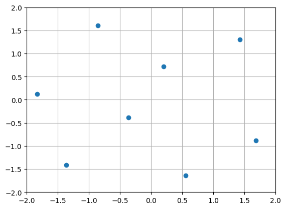
Let’s first create a Latin hypercube sampling (LHS). We will discuss later why it is superior to random sampling (Learn more about |LHS| and orthogonal sampling here). We will first define a ParameterSpace with uniform distribution using the function create_continuous_uniform_space and then use the OrthogonalSamplingDesigner class to generate the Design of Experiments (DoE) and plot the result.

from experiment_design import create_continuous_uniform_space, OrthogonalSamplingDesigner
import matplotlib.pyplot as plt

    # Define the parameter space
space = create_continuous_uniform_space([-2., -2.], [2., 2.])

    # Generate a design of experiments
doe = OrthogonalSamplingDesigner().design(space, sample_size=8)

    # Plot the generated samples
plt.scatter(doe[:, 0], doe[:, 1])
plt.xlim([-2, 2])
plt.ylim([-2, 2])
plt.grid()

This will result in a plot similar to the following:

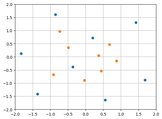
Since we are generating randomized designs, the placement of the samples may be different in each run. Imagine that we are interested in a smaller space and want to generate more samples there, while maximizing the minimum distance between samples. The old_sample keyword argument allows users to provide previously generated samples, ensuring the new samples fill the portions of the space that are not covered by the old samples.

    # Define a new parameter space
space2 = create_continuous_uniform_space([-1., -1.], [1., 1.])

    # Generate a new design of experiments by extending the old one
doe2 = OrthogonalSamplingDesigner().design(space2, sample_size=8, old_sample=doe)

    # Plot the new samples
plt.scatter(doe2[:, 0], doe2[:, 1])

The resulting samples, displayed in orange, fill the empty space as much as possible without inducing additional correlation. Moreover, the LHS scheme is kept within the newly defined space boundaries \([-1, 1]^2\) in this case and whenever it’s possible.

To learn more about generating space-filling DoE for non-uniform and possibly correlated variables, proceed to the next section.