Experiment Design via Orthogonal Sampling
Suppose we want to conduct experiments and have complete control over the values of the input parameters. There are a number of approaches to select values, including
and others. Although all of these designs have beneficial properties such as being space-filling or efficient concerning certain optimization criteria, they do not account for parameter uncertainty.
However, modeling uncertainty is often necessary for tasks such as statistical inference based on a sample. Orthogonal design allows us to model the parameter uncertainties while providing experiment designs with higher quality compared to random sampling with respect to space-filling properties. Since orthogonal sampling is a generalization of Latin hypercube sampling ( LHS ) to non-uniform variables, we will begin by describing how an experiment can be designed using LHS and why it is superior to random sampling.
Latin hypercube sampling
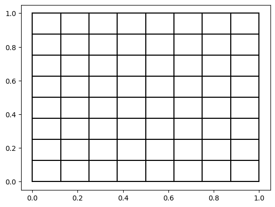
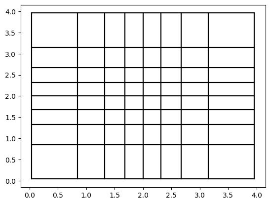
LHS is a generalization of the Latin sphere to higher dimensional spaces, first proposed by McKay et al. (1979). Three steps are required to generate an LHS. For visualization purposes, we will be using a two dimensional space with the bounds \([0, 1]^2\). Before generating the design, we need to decide how many samples we will need. For now let’s create 8 samples. First, we partition the space into small squares (or hypercubes, if we had more than two dimensions), such that each dimension is divided into 8 parts. We will refer to these hypercubes as bins. We can visualize this as follows:
import matplotlib.pyplot as plt
import numpy as np

bin_edges = np.linspace(0, 1, 9)  # we need 9 lines to represents 8 bins
plt.figure()
for x in bin_edges:
    plt.plot([x, x], [0, 1], c="k")
    plt.plot([0, 1], [x, x], c="k")
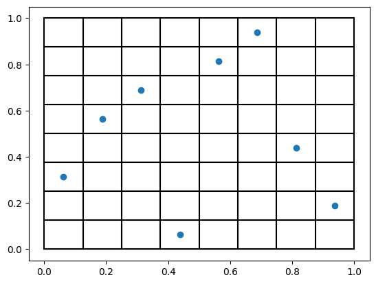
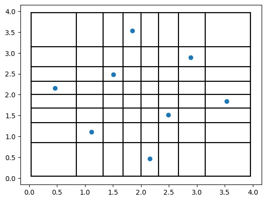
Next, we place each sample such that each bin is occupied only once in each dimension. This is quite easy to implement,
but since we are show casing the capabilities of experiment-design, let’s use it here.
from experiment_design import create_continuous_uniform_space, OrthogonalSamplingDesigner

np.random.seed(1337)
space = create_continuous_uniform_space([0.0, 0.0], [1., 1.])
designer = OrthogonalSamplingDesigner(inter_bin_randomness=0.0)
doe = designer.design(space, sample_size=8, steps=1)
plt.scatter(doe[:, 0], doe[:, 1], label="Init. design")
There are a few important details in the above code so let’s walk line by line. After importing the necessary modules,
we first set a random seed. This is important for reproducibility. Given the same inputs and seed, we will always
generate the same design on the same machine. Next, we define a two dimensional parameter space (ParameterSpace)
within the bounds \([0, 1]^2\). In general, bounds need not be equal. They can be any finite values, provided the lower
bound for a variable is smaller than its corresponding upper bound.
Following, we initiate an OrthogonalSamplingDesigner
with the parameter. inter_bin_randomness=0.. This controls the randomness of the placement of samples within the
bins. A value of 0.0 places the samples exactly in the middle of the bins, whereas a value of 0.8 (default) would lead to
placing samples anywhere between \([-0.4 \delta, 0.4 \delta]\) within the bin, where \(\delta\) is the bin size,
here \(\delta=1/8=0.125\). Finally, we generate a DoE using only 1 step, i.e. skipping any optimization for now, that we
would do normally and plot the result.
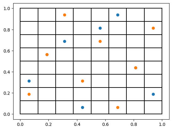
Final step is not mandatory, but it improves the DoE quality a lot, as proposed by Joseph et al. (2008):
Optimize the samples using simulated annealing by switching the values of samples along each dimension.
Simulated annealing is a stochastic optimization algorithm inspired by the annealing process in metallurgy.
It is particularly effective for optimizing black-box objective functions,
especially in cases where gradients are unavailable or the solution space is highly non-linear and complex.
We will talk about the optimization objectives used in experiment-design later.
Switching values does not violate the LHS rules; each bin remains occupied only once.
This is done automatically in experiment-design unless we turn it off as we did before.
In order to start from the same DoE, we set the same seed but use the default number of steps.
np.random.seed(1337)
doe2 = designer.design(space, sample_size=8)
plt.scatter(doe2[:, 0], doe2[:, 1], label="Final design")
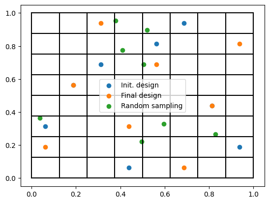
Finally, we create some random samples to serve as a baseline. We can do this using experiment-design too.
Implicitly, there is also some search for the random sampler, where we evaluate the random DoE on the same set of
objectives as before and choose the one that achieves the best results. For the purposes of this document, we will
deactivate the optimization by setting. steps=1 as we did before.
from experiment_design import RandomSamplingDesigner

doe3 = RandomSamplingDesigner().design(space, sample_size=8, steps=1)
plt.scatter(doe3[:, 0], doe3[:, 1], label="Random sampling")
plt.legend()
Quality metrics
We can look at two metrics to evaluate the quality of the DoE; the minimum pairwise distance to evaluate its
space-filling properties as well as the correlation coefficient \(|\Delta\rho|\) between the variables. We use
scipy.spatial.distance.pdist(doe).min() to compute the pairwise distance metric and
np.abs(np.corrcoef(doe, rowvar=False)[0, 1]) for the correlation error. Results are given below.
DoE |
Min. distance |
\(|\Delta\rho|\) |
|---|---|---|
doe |
0.18 |
0.00 |
doe2 |
0.35 |
0.14 |
doe3 |
0.13 |
0.19 |
Initial LHS has no correlation error, although the optimized LHS induces some correlation but it almost doubles the minimum pairwise distance, filling the parameter space much better. This is partially due to the default objective we use in experiment-design, where we put 9 times more emphasis on the space filling properties compared to the correlation error. Nevertheless, as we will see later, we can change the weights we use arbitrarily and even supply a custom objective function. In any case, both LHS designs achieve better metrics compared to random sampling.
Having demonstrated how LHS samples are generated and their quality compared to random sampling, we now discuss orthogonal sampling and its usefulness for statistical inference.
Orthogonal sampling
It is straightforward to generalize LHS to orthogonal sampling, where we generate an LHS design in \([0, 1]^d\), in a d-dimensional parameter space, which we interpret as probabilities and use the inverse CDF functions of the marginal variables to map them to actual values. Let’s see this in action in a 2-dimensional space for visualization purposes. Let’s define two Gaussian variables \(X_1, X_2 \sim \mathcal{N}(2, 1)\) with a means \(\mu_1 = \mu_2 = 2\) and a variances \(\sigma_1 = \sigma_2 = 1\). Again, we start by partitioning the probability space into 8 intervals to generate 8 samples, which yields the same bounds as before. Next, we map them back to the original space. The code looks like this:
import matplotlib.pyplot as plt
import numpy as np
from scipy import stats

from experiment_design import ParameterSpace, OrthogonalSamplingDesigner

space = ParameterSpace(variables=[stats.norm(2, 1) for _ in range(2)],
                       infinite_bound_probability_tolerance=2.5e-2)
probability_bin_edges = np.linspace(0, 1, 9)
# create an array of probabilities, where each column represents a variable
probability_bin_edges = np.c_[probability_bin_edges, probability_bin_edges]
# Below line calls scipy_distribution.ppf for each variable under the hood
bin_edges = space.value_of(probability_bin_edges)
bin_edges[0] = space.lower_bound
bin_edges[-1] = space.upper_bound

plt.figure()
for x in bin_edges:
    plt.plot([x[0], x[0]], [bin_edges[0, 1], bin_edges[-1, 1]], c="k")
    plt.plot([bin_edges[0, 0], bin_edges[-1, 0]], [x[1], x[1]], c="k")
Notice the infinite_bound_probability_tolerance variable in the above. Since the normal distribution has
infinite bounds, i.e. unbounded support, the outer most grid lines for each dimension corresponding to the probabilities
0 and 1 would also be at infinity. In order to still provide a finite bound for practical applications and thus enforce
finite bin sizes for all dimensions, we define the parameter infinite_bound_probability_tolerance, which is set to
1e-6 by default. In this case, we set it to a much larger value for visualization purposes.
Next, we generate an optimized DoE starting from the same initial solution as before.
Notice that, besides the bin sizes, the placement of the samples is also different compared to the above example.
The random effects are negligible in this case due to the small number of samples and the value of inter_bin_randomness.
Although the probability space is the same as in the LHS example,
the reason for the difference in results is the varying bin sizes in the parameter space,
which yield an optimal placement that differs from the uniform case.
np.random.seed(1337)
designer = OrthogonalSamplingDesigner(inter_bin_randomness=0.)
doe = designer.design(space, sample_size=8)
plt.scatter(doe[:, 0], doe[:, 1])
Why should you use orthogonal sampling?
So far, we have only created colorful plots but you might wonder, why we need this much effort when random sampling would also yield a DoE with the appropriate distribution. Let us look at a practical use case to show case the actual benefit of using orthogonal sampling.
Let \(X_1, X_2\) follow the same distribution as above and let \(Y = X_1 + X_2\) be a random variable, for which
we want to estimate the expectation \(\mathbb{E}[Y] = \mu_Y\). Using the linear relationship above and due to the
normal distribution of the variables and assuming independence, we can infer that \(Y \sim \mathcal{N}(4, \sqrt{2})\)
and thus \(\mu_Y=4\). For the purposes of this demonstration, assume that the exact relationship between \(X_1, X_2\)
and \(Y\) are not known but we can use the black-box function \(Y = f(X_1, X_2)\) to estimate \(\mu_Y\) from
samples. We could use the following code for the estimation using OrthogonalSamplingDesigner and RandomSamplingDesigner
import matplotlib.pyplot as plt
import numpy as np
from scipy import stats

from experiment_design import ParameterSpace, OrthogonalSamplingDesigner, RandomSamplingDesigner

def f(x: np.ndarray) -> np.ndarray:
    # implementation using array operations
    return x.sum(axis=1)

space = ParameterSpace(variables=[stats.norm(2, 1) for _ in range(2)])
osd = OrthogonalSamplingDesigner()
rsd = RandomSamplingDesigner()

np.random.seed(1337)
doe_os = osd.design(space, sample_size=32)
doe_rs = rsd.design(space, sample_size=32)

y_os = f(doe_os)
y_rs = f(doe_rs)

print("Orthogonal Sampling:", np.mean(y_os))  # 4.0112
print("Random Sampling:", np.mean(y_rs))  # 4.1066
Now you could say, this is just luck, which would make me happy because it means that you are paying attention. Yes, this could be due to pure luck. In order to provide a more convincing demo without going into the theoretical details that can be found in the linked literature, let us create a convergence plot.
results_os, results_rs = [], []
sample_sizes = list(range(8, 136, 8))
for sample_size in sample_sizes:
    doe_os = osd.design(space, sample_size=sample_size)
    doe_rs = rsd.design(space, sample_size=sample_size)

    y_os = f(doe_os)
    y_rs = f(doe_rs)

    results_os.append(np.mean(y_os))
    results_rs.append(np.mean(y_rs))

plt.plot(sample_sizes, results_rs, label="Random sampling")
plt.plot(sample_sizes, results_os, label="Orthogonal sampling")
plt.grid();plt.legend()
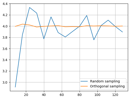
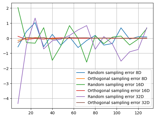
As you can see, orthogonal sampling achieves a much smaller error throughout. We can see a similar difference in higher dimensions. Analytically, we know that \(\mu_Y = 2d\), where \(d\) is the number of dimensions.
plt.figure()
for dimensions in [8, 16, 32]:
    space = ParameterSpace(variables=[stats.norm(2, 1) for _ in range(dimensions)])
    errors_os, errors_rs = [], []
    for sample_size in sample_sizes:
        doe_os = osd.design(space, sample_size=sample_size)
        doe_rs = rsd.design(space, sample_size=sample_size)

        y_os = f(doe_os)
        y_rs = f(doe_rs)

        errors_os.append(np.mean(y_os) - 2 * dimensions)
        errors_rs.append(np.mean(y_rs) - 2 * dimensions)

    plt.plot(sample_sizes, errors_rs, label=f"Random sampling error {dimensions}D")
    plt.plot(sample_sizes, errors_os, label=f"Orthogonal sampling error {dimensions}D")
plt.grid();plt.legend()
Warning
Note that th.. code above may take a long time to run. The reason behind this is the number of optimization steps
taken by OrthogonalSamplingDesigner especially in lower sample setting (\(\leq 128\)) as the optimization has a
high impact on the quality of the resulting DoE. You can choose a smaller step value
(the default is 20000 for sample_size \(\leq 128\) and 2000 otherwise) or even set it to 1 or less to avoid
any optimization, which would accelerate the run time significantly.
Finally, the reduced estimation error becomes even more significant for non-linear and multimodal functions. For example, consider the Ackley function with its recommended default values. We choose this function due to its multimodality and complexity despite being 2 dimensional. It is difficult to compute its expectation, but we can approximate it with a very high number of random samples.
def ackley(x: np.ndarray) -> np.ndarray:
    y = -20 * np.exp(-0.2 * np.sqrt(np.sum(x**2, axis=1) / x.shape[1]))
    y -= np.exp(np.sum(np.cos(2 * np.pi * x), axis = 1) / x.shape[1])
    return y + 20 + np.exp(1)

space = ParameterSpace(variables=[stats.weibull_min(1),
                                  stats.weibull_min(2, loc=-2, scale=2)])
large_doe = rsd.design(space, sample_size=100_000, steps=1)
y = ackley(large_doe)
print("Mean:", np.mean(y))   # 5.1
print("Std. Err.", np.std(y, ddof=1) / np.sqrt(y.shape[0]))  # 0.007
When we have a more limited sample budget, using orthogonal sampling leads to more accurate estimates.
np.random.seed(1337)
doe_os = osd.design(space, sample_size=64)
doe_rs = rsd.design(space, sample_size=64)

print("Orthogonal Sampling:", np.mean(ackley(doe_os)))  # 5.2
print("Random Sampling:", np.mean(ackley(doe_rs)))  # 5.6
In summary, orthogonal sampling increases estimation accuracy and reduces estimation variance when conducting statistical inference. It also creates space-filling samples that improves the exploration and benefit machine learning models similar to LHS.
Why choose experiment-design?
So far, we have been discussing the advantages of LHS and orthogonal sampling over random sampling. However,
experiment-design is not the only library to provide this functionality. For instance,
pyDOE is a popular library that provides the capability to create an LHS,
even using similar optimization criteria as experiment-design. Nevertheless, users need to choose between either
optimizing for the minimum distance or the maximum correlation error. Moreover, we could use this capability to create
an orthogonal sampling simply by generating an LHS in \([0, 1]^d\) and using the values as probabilities.
In short, the benefits of using experiment-design over other choices for generating LHS and orthogonal design are
Generation of space-filling DoE with low correlation error
Flexible optimization criteria for DoE generation
Capability to simulate correlations while maintaining space-filling properties
Extending LHS and orthogonal sampling while adhering to the Latin hypercube scheme as much as possible
The following sections demonstrate these capabilities in detail.
Generate high quality DoE with built-in or custom metrics
Before looking at further features, let’s put this hypothesis into test and do a small comparison. Note that you need to install pyDOE to run the following code.
import numpy as np
from scipy import stats

from pyDOE3 import lhs
from experiment_design import ParameterSpace, OrthogonalSamplingDesigner

sample_size = 64

np.random.seed(1337)
doe_maximin = lhs(2, sample_size, "maximin", 20_000)

np.random.seed(1337)
doe_corr = lhs(2, sample_size, "correlation", 20_000)

np.random.seed(1337)
doe_lhsmu = lhs(2, sample_size, "lhsmu", 20_000)

space = ParameterSpace(variables=[stats.uniform(0, 1) for _ in range(2)])
np.random.seed(1337)
doe_ed = OrthogonalSamplingDesigner().design(space, sample_size, steps=20_000)
As before (see Quality metrics), we will compute the correlation error as well as the minimum pairwise distance.
DoE |
Min. distance |
\(|\Delta\rho|\) |
|---|---|---|
doe_maximin |
0.05 |
0.17 |
doe_corr |
0.02 |
6e-6 |
doe_lhsmu |
0.02 |
0.27 |
doe_ed |
0.10 |
1e-4 |
In comparison, the minimum pairwise distance for the DoE generated by the experiment-design is much larger, which
represents better space filling properties. Moreover, also the correlation error is better for experiment-design
compared to all results generated by pyDOE3 except when using correlation error as the target, which achieves the worst
the minimum pairwise distance. In general, the correlation error achieved by experiment-design is negligibly small
for most practical purposes. Nevertheless, we can improve the result further by providing a custom scoring function;
a feature that is not present in other libraries. Let’s see it in action.
def correlation_scorer_factory(*args, **kwargs):
    def _correlation_scorer(doe: np.ndarray) -> float:
        return -1. * np.max(
            np.abs(np.corrcoef(doe, rowvar=False) - np.eye(doe.shape[1]))
        )
    return _correlation_scorer

designer = OrthogonalSamplingDesigner(scorer_factory=correlation_scorer_factory)
np.random.seed(1337)
doe_ed_corr = designer.design(space, sample_size, steps=20_000)
Using the above code, we achieve a maximum correlation error of 5e-7, a score lower than the best score achieved with
pyDOE. Note that correlation_scorer_factory is essentially a simplified version of
MaxCorrelationScorerFactory which is one of the two weighted objectives used by default. This implementation was chosen to
demonstrate the ability to define custom scoring functions, including those tailored to specific domains and even penalty functions
representing constraints. Support for actual constraints is currently not on our road map. If you are interested in this functionality,
please create an issue on github <https://github.com/canbooo/experiment-design>.
However, mapping probabilities to the actual parameter space may lead to worse results. Let’s consider a
space with two non-normal variables. We can map the probabilities using the ParameterSpace.value_of method.
space = ParameterSpace(variables=[stats.lognorm(0.3), stats.uniform(-1, 2)])

doe_maximin = space.value_of(doe_maximin)
doe_corr = space.value_of(doe_corr)
doe_lhsmu = space.value_of(doe_lhsmu)
# Below is just for the sake of comparability
doe_ed = space.value_of(doe_ed)
np.random.seed(1337)
# This is how we would actually create a DoE in this space:
doe_ed_new = OrthogonalSamplingDesigner().design(space, sample_size, steps=20_000)
Results are given in the table below. It can be seen that first optimizing and than matching the probabilities leads to
a much higher correlation error and smaller pairwise distance even for the DoE with good metrics in the probability
space. Therefore, using pyDOE3 for non-uniform use cases may lead to worse metrics.
DoE |
Min. distance |
\(|\delta\rho|\) |
|---|---|---|
doe_maximin |
0.05 |
0.18 |
doe_corr |
0.01 |
0.02 |
doe_lhsmu |
0.03 |
0.11 |
doe_ed |
0.08 |
0.02 |
doe_ed_new |
0.12 |
1e-5 |
Extend experiments adaptively
Finally, one of the most novel features of experiment-design is the ability to extend an LHS and an orthogonal sampling
by generating new samples that adhere to the Latin hypercube scheme when possible
(See Bogoclu (2022)).
One use case of this feature is to extend the experiments in regions with interesting or unsatisfying results. Let’s
consider the same problem as above, where we wanted to estimate the mean of the Ackley function.
import matplotlib.pyplot as plt
import numpy as np
from scipy import stats

from experiment_design import ParameterSpace, OrthogonalSamplingDesigner


def ackley(x: np.ndarray) -> np.ndarray:
    y = -20 * np.exp(-0.2 * np.sqrt(np.sum(x**2, axis=1) / x.shape[1]))
    y -= np.exp(np.sum(np.cos(2 * np.pi * x), axis = 1) / x.shape[1])
    return y + 20 + np.exp(1)


np.random.seed(1337)
space = ParameterSpace(variables=[stats.weibull_min(1),
                                  stats.weibull_min(2, loc=-2, scale=2)],)

designer = OrthogonalSamplingDesigner()

doe = designer.design(space, sample_size=8)
results = [np.mean(ackley(doe))]
sample_sizes = [8]

for new_sample_size in [8, 16, 32, 64, 128]:
    new_doe = designer.design(space, sample_size=new_sample_size, old_sample=doe)
    doe = np.append(doe, new_doe, axis=0)
    results.append(np.mean(ackley(doe)))
    sample_sizes.append(doe.shape[0])

plt.plot(sample_sizes, results)
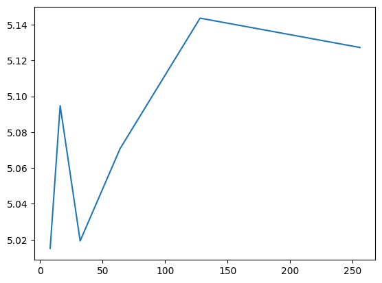
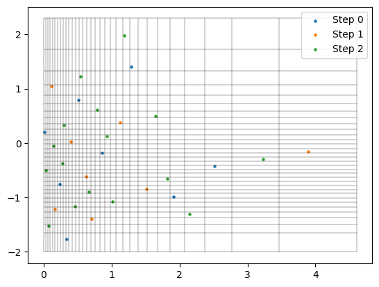
It can be seen that the value converges to the estimate made by \(10^5\) random samples. Notice that we are doubling the sample size at each step. This is not mandatory but it guarantees that the resulting DoE is an LHS. Let’s visualize the first few iterations as visualizing all 256 samples is not very nice on the eyes.
space = ParameterSpace(variables=[stats.weibull_min(1),
                                  stats.weibull_min(2, loc=-2, scale=2)],
                       infinite_bound_probability_tolerance=1e-2)  # just for vis. purposes

probability_bin_edges = np.linspace(0, 1, 33)
probability_bin_edges = np.c_[probability_bin_edges, probability_bin_edges]
# Below line calls scipy_distribution.ppf for each variable under the hood
bin_edges = space.value_of(probability_bin_edges)
bin_edges[0] = space.lower_bound
bin_edges[-1] = space.upper_bound

plt.figure()
for x in bin_edges:
    plt.plot([x[0], x[0]], [bin_edges[0, 1], bin_edges[-1, 1]], c="k", linewidth=0.25)
    plt.plot([bin_edges[0, 0], bin_edges[-1, 0]], [x[1], x[1]], c="k", linewidth=0.25)

plt.scatter(doe[:sample_sizes[0], 0], doe[:sample_sizes[0], 1], label="Step 0", s=5)
for i, (old_size, new_size) in enumerate(zip(sample_sizes[:2], sample_sizes[1:3])):
    plt.scatter(doe[old_size:new_size, 0], doe[old_size:new_size, 1], label=f"Step {i + 1}", s=5)

plt.legend()
Here are some further visualizations of DoE extensions. Note that the space in which we extend the DoE does not need to match the original space, and we are not required to double the sample size.